Visualisation of Tree-based Phylogenetic Networks with ggret

ggret is an R package for the visualization of tree-based phylogenetic networks. Its builds on and extends ggplot2 and ggtree and aims to be compatible with these packages. For more details about ggtree’s functionalities, please see the ggtree vignette here: https://yulab-smu.top/treedata-book/

Installation

As a first step, we recommend getting ggplot2 from CRAN and ggtree from Bioconductor if you haven’t done this previously. The ggret package is available via GitHub and can be installed with the remotes package.

# Install ggplot2
install.packages("ggplot2")

# Install ggtree
if (!require("BiocManager", quietly = TRUE))
    install.packages("BiocManager")

BiocManager::install("ggtree")

# Install ggret
if (!requireNamespace("remotes", quietly = TRUE))
  install.packages("remotes")
remotes::install_github("grdspcht/ggret", dependencies = TRUE, build_vignettes = TRUE)

Parsing network formats

ggret provides parsing functions building upon ape::read.tree and treeio::read.beast for reading extended Newick and BEAST2 NEXUS files with network blocks. The input data is stored in evonet or treedata objects and can be used for plotting and further analysis.

library(ggret)

#read_enewick parses extended Newick format and generates an evonet object. 
retfile_nwk <- system.file("extdata" , "retnet.nwk", package = "ggret", mustWork = TRUE)
retnet_evonet <- ggret::read_enewick(retfile_nwk)

#read_beast_retnet parses BEAST2 NEXUS files and generates a treedata object.
retfile_nexus <- system.file("extdata" , "retnet.nexus", package = "ggret", mustWork = TRUE)
retnet_treedata <- ggret::read_beast_retnet(retfile_nexus)

For the next step of the tutorial, we will instead use the retnet_treedata object which also comes with this package. It is a treedata object corresponding to a (summary) phylogenetic network simulated with the BEAST2 package Bacter containing various node metadata.

Plotting a basic phylogenetic network

ggret is the central function of this package. In a simple call without additional arguments it only plots a visual representation of the phylogenetic network.

We first use the original ggtree function to plot the backbone tree of the retnet object

ggtree::ggtree(retnet_evonet)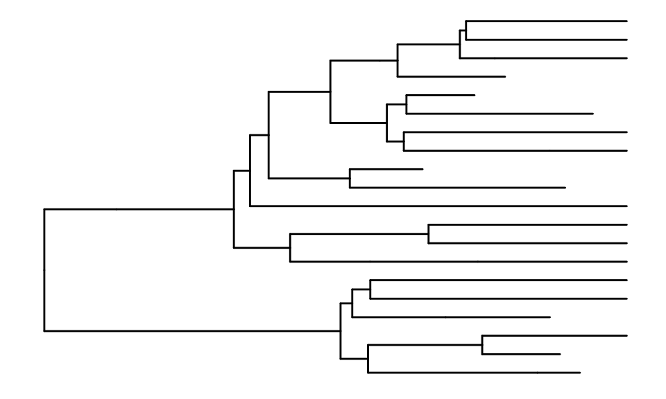

We now plot the entire network, including reticulation edges, using the ggret function.

ggret::ggret(retnet_evonet)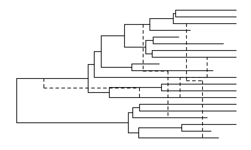

Changing the aspect of reticulation edges

The ggret functions can take different arguments to change the aspect of reticulation edges.

# Reticulation edges displayed as red dotted lines, in a "snake" shape
p1 <- ggret::ggret(retnet_evonet, retcol = "red", retlinetype = 3)
# Reticulation edges displayed as blue solid lines, in a straight shape and with arrow heads
p2 <- ggret::ggret(retnet_evonet, retcol = "blue", retlinetype = 1, arrows = T, rettype = "straight")
# Plot
plot(p1)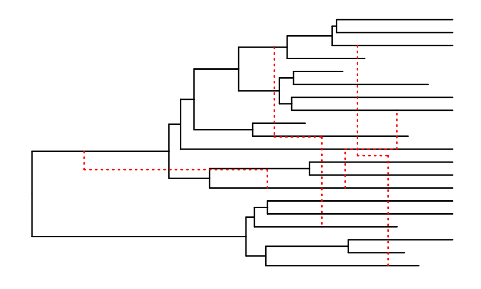

plot(p2)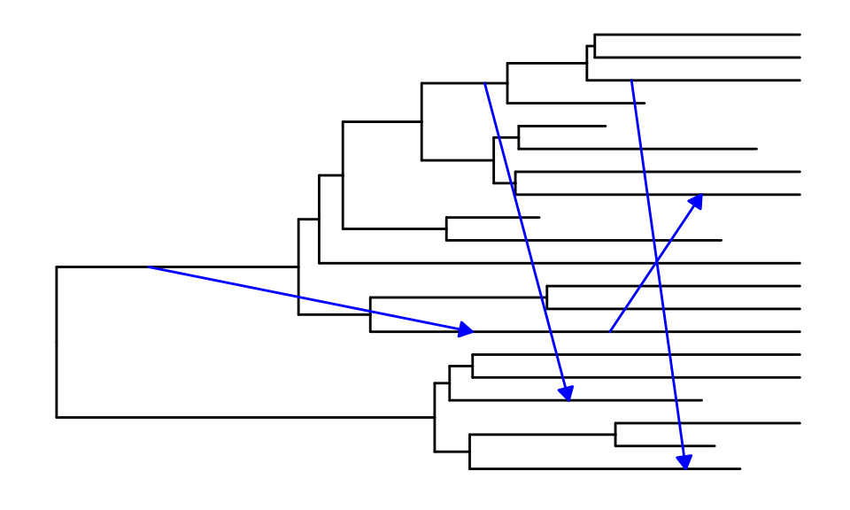

Annotating a phylogenetic network

Adding geom_tiplab and geom_nodelab from ggtree to our previous call allows us to annotate the network with metadata that is stored in the retnet object.

Here is an example to add tip labels and posterior support values at the nodes. Note that we have to expand the x axis limits to make the tip labels visible.

ggret::ggret(retnet_treedata) + 
  ggtree::geom_tiplab() +
  ggtree::geom_nodelab(aes(label = round(posterior,2)), vjust = -0.25, hjust = 1.2, size = 3) +
  ggplot2::expand_limits(x = 23000)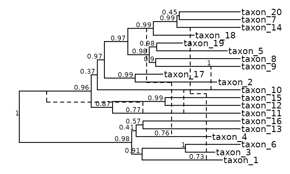

Here is another example in which we add a time axis to the plot, as well as the node heights’ 95% highest posterior density intervals represented by bars. This example requires the phytools package.

# Get the tMRCA of the tree and define time points to display in the time axis in years BP
library(phytools)
tmrca <- phytools::nodeHeights(retnet_treedata@phylo) %>% max
xticks_BP <- c(20000,15000,10000,5000,0)

# Plot the network
ggret::ggret(retnet_treedata) +
  ggtree::theme_tree2() +
  ggtree::geom_range(aes(range = "height_95_HPD"), color = "grey50", alpha = .6, size = 1.5) +
  ggplot2::scale_x_continuous(breaks = tmrca - xticks_BP, labels = xticks_BP) +
  ggplot2::xlab("Years before present")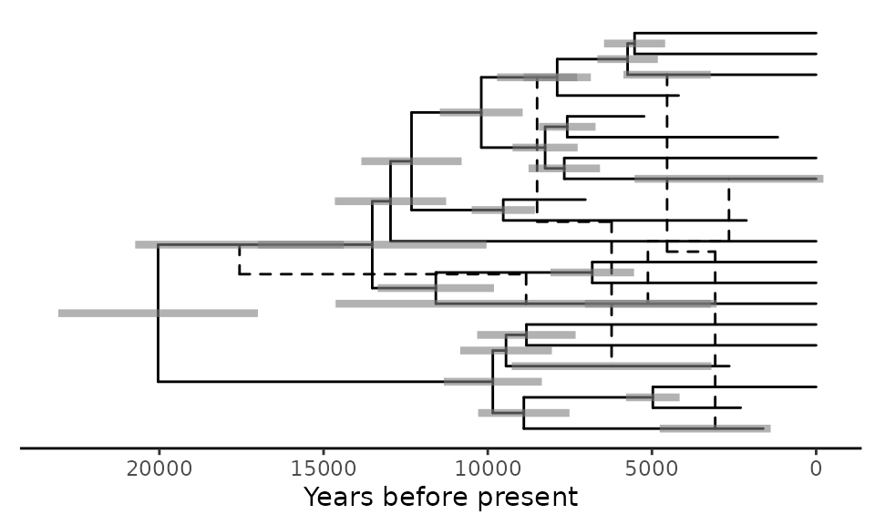

Adding color to your network

With group_clade we can define clades within our network and then use aes to color them accordingly. group_clade assigns clade information to all nodes descending from the MRCA of tips specified in the nodes argument. The value taken is specified in the cladename argument and is added as a clade attribute in the evonet object and, in addition, as a Clade column in the data component of tree data objects if the addtotreedata argument is set to true.

# Define clades using the group_clade function
retnet_treedata %>%
  ggret::group_clade(nodes = c("taxon_10", "taxon_20"), cladename = "A", addtotreedata = T) %>%
  ggret::group_clade(nodes = c("taxon_11", "taxon_15"), cladename = "B", addtotreedata = T) %>%
  ggret::group_clade(nodes = c("taxon_1", "taxon_16"), cladename = "C", addtotreedata = T) ->
  retnet_clade

# Plot network with colored clades
ggret::ggret(retnet_clade, aes(color = Clade))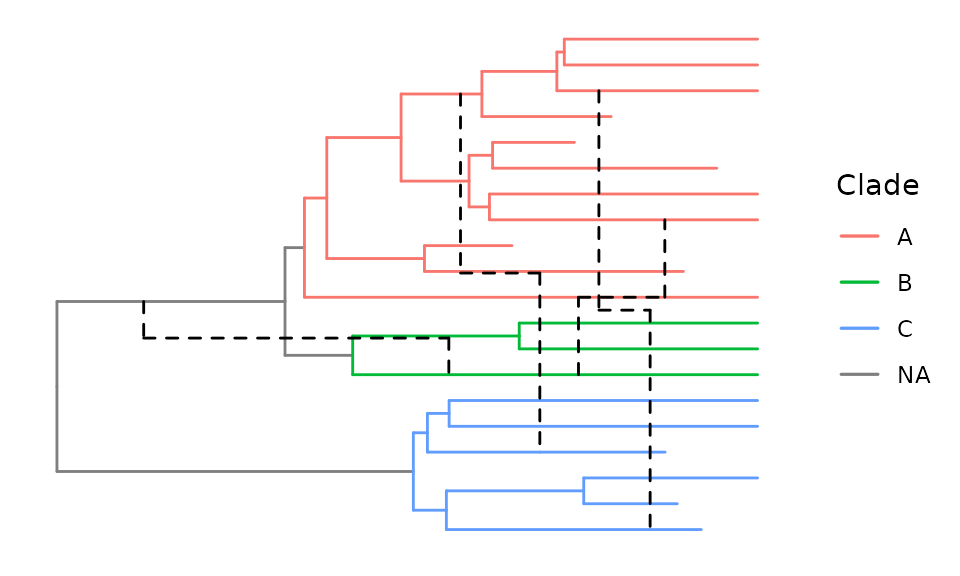

Citations

If you use ggret, please cite the associated publication as well as the original ggtree publication:

ggret publication to be added
G Yu, DK Smith, H Zhu, Y Guan, TTY Lam^*. ggtree: an R package for visualization and annotation of phylogenetic trees with their covariates and other associated data. Methods in Ecology and Evolution. 2017, 8(1):28-36. doi: 10.1111/2041-210X.12628.